43 format data labels pane excel

› advanced_excel › advancedAdvanced Excel - Leader Lines - Tutorials Point Step 3 − Move the data label. The Leader Line automatically adjusts and follows it. Format Leader Lines. Step 1 − Right-click on the Leader Line you want to format. Step 2 − Click on Format Leader Lines. The Format Leader Lines task pane appears. Now you can format the leader lines as you require. Step 3 − Click on the icon Fill & Line. Format Chart Axis in Excel - Axis Options Analyzing Format Axis Pane. Right-click on the Vertical Axis of this chart and select the "Format Axis" option from the shortcut menu. This will open up the format axis pane at the right of your excel interface. Thereafter, Axis options and Text options are the two sub panes of the format axis pane.

How to: Display and Format Data Labels - DevExpress Specify the Position of Data Labels; Apply Number Format to Data Labels; Create a Custom Label Entry; Add Data Labels to the Chart. Basic settings that specify the contents, position and appearance of data labels in the chart are defined by the DataLabelOptions object, accessed by the ChartView.DataLabels property. Use the object's properties to display data labels for all series in the current chart view and specify what information should appear in each label.

Format data labels pane excel

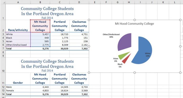
support.microsoft.com › en-us › officeDesign the layout and format of a PivotTable You can add a field only once to either the Report Filter, Row Labels, or Column Labels areas, whether the data type is numeric or non-numeric. If you try to add the same field more than once — for example to the Row Labels and the Column Labels areas in the layout section — the field is automatically removed from the original area and put ... Format a table in Excel and naming tips - Power Apps How to format a table in Excel You can convert your data to a table by selecting Format as Table in the Home tab of Excel. You can also create a table by selecting Table on the Insert tab. To find your table easily, go to Design under Table Tools, and rename your table. Pie Chart in Excel - Inserting, Formatting, Filters, Data Labels Right click on the Data Labels on the chart. Click on Format Data Labels option. Consequently, this will open up the Format Data Labels pane on the right of the excel worksheet. Mark the Category Name, Percentage and Legend Key. Also mark the labels position at Outside End. This is how the chark looks. Formatting the Chart Background, Chart Styles

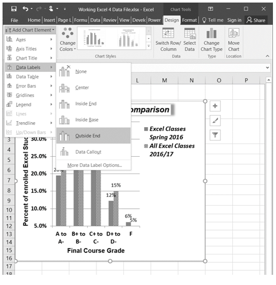
Format data labels pane excel. How to ☝️Make a Pie Chart in Excel (Free Template) In the task pane that appears, do the following to spruce up your data labels: Navigate to the "Label Options" tab. Under "Label Options," select "Category Name" to display the product categories next to the actual values. Under "Label Position," click "Outside End" to push the labels outside the pie chart. How to Print Labels from Excel - Lifewire Select Mailings > Write & Insert Fields > Update Labels . Once you have the Excel spreadsheet and the Word document set up, you can merge the information and print your labels. Click Finish & Merge in the Finish group on the Mailings tab. Click Edit Individual Documents to preview how your printed labels will appear. Select All > OK . How to Create A 3-D Pie Chart in Excel [FREE TEMPLATE] The data in the table is pretty self-explanatory, so move on to the nitty-gritty. Here's the easiest way to create a 3-D pie chart: Select any cell in the data table ( A1:A6 ). Switch to the Insert tab. Choose " Insert Pie or Doughnut Chart. ". Click " 3-D Pie. ". Just a few clicks are your 3-D chart is ready to go: Usage, Types, Scatter Chart - Excel Unlocked To add the Data Labels on the chart:- Click on the chart On the top right corner of chart, a + icon would appear. Click on it. Mark the Data Labels from the menu and click on More Options This opens the Format Data Labels Pane on the right of the excel window. From there mark the X and Y coordinates to be displayed via the Data Labels.

Custom Chart Data Labels In Excel With Formulas Select the chart label you want to change. In the formula-bar hit = (equals), select the cell reference containing your chart label's data. In this case, the first label is in cell E2. Finally, repeat for all your chart laebls. If you are looking for a way to add custom data labels on your Excel chart, then this blog post is perfect for you. Mailing Labels in Word from an Excel Spreadsheet - W3codemasters To apply the formatting to all of the labels, go to the Mailings tab and hit 'Update Labels '. Navigate to the 'Mailings' page to conduct the merging. In the Finish group, select the 'Finish & Merge' box. From the drop-down menu, choose 'Edit Individual Documents. A tiny pop-up window with the title "Merge to New Document" will appear. How to ☝️Make a Gantt Chart in Excel - SpreadsheetDaddy 2. In the Format Cells dialog box, under " Category ," choose " Custom .". 3. In the " Type " field, enter mmm d to set a custom date format that will make it a lot easier to read the chart. Once there, here's how the dates you modified should look: Step 2. Prepare the Gantt Chart Data. github.com › dbeaver › dbeaverData View and Format · dbeaver/dbeaver Wiki · GitHub Oct 11, 2021 · Configuring Numeric and Time Data Formats. You can specify the exact format of Time, Timestamp, Date, and Number data used in the currently open database or globally. To specify a format, right-click any cell in the table and, on the context menu, click View/Format -> Data formats. The Properties window opens displaying the Data Formats page:

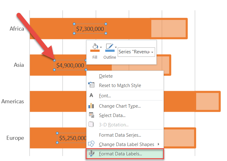
docs.microsoft.com › office-file-format-referenceFile format reference for Word, Excel, and PowerPoint ... Sep 30, 2021 · The Excel 5.0/95 Binary file format. .xlsb : Excel Binary Workbook : The binary file format for Excel 2019, Excel 2016, Excel 2013, and Excel 2010 and Office Excel 2007. This is a fast load-and-save file format for users who need the fastest way possible to load a data file. Supports VBA projects, Excel 4.0 macro sheets, and all the new ... mgconsulting.wordpress.com › 2013/12/09 › add-a-dataAdd a Data Callout Label to Charts in Excel 2013 Dec 09, 2013 · You can also apply advanced formatting by right clicking the label and selecting Format Data Labels. This will open a task pane on the right side of your screen with options for formatting position, number formatting, and more. MG Consulting is a software consulting and training company located in the Boston area. For information about Excel ... How to Use the Navigation Pane in Microsoft Excel Navigation. When you first open the Navigation pane, you'll see all of the sheets in the workbook listed in order. Simply click a sheet name in the list to move directly to it in the workbook. If you select a sheet tab, you'll also see the sheet name in bold font in the pane. Each sheet in the list also has an arrow to the left allowing you ... Bubble Chart in Excel-Insert, Working, Bubble Formatting - Excel Unlocked Click on More Options in the Data Labels sub menu. This opens the Format Data Labels Pane at the right of the excel window. Open the Label Options and make the checkbox for Value from Cells. Make sure that the rest of the checkboxes in the label options are unmarked. Select the range A2:A6 and click Ok to add it to data labels.

Excel 2016 charts: How to use the new Pareto, Histogram, and Waterfall formats | PCWorld

2 Cara Mengubah Format Angka Menjadi Persentase Dalam Excel 1. Mengubah Angka ke Persen Melalui Tab Home. Cara yang pertama untuk mengubah angka menjadi persen adalah melalui menu Number Format yang ada pada Tab Home. Pada Tab Home tersebut terdapat kelompok menu Number dimana didalamnya terdapat sub menu Number Format. Pada sub menu Number Format tersebut ada banyak format yang dapat digunakan mulai ...

Excel 2013 Tutorial Formatting Data Labels Microsoft Training Lesson 28.6 - YouTube

Getting started with formatting report visualizations - Power BI Select the visual to make it active and open the Formatting pane. Scroll down to Data labels and Total labels. Data labels is On and Total labels is Off. Turn Data labels Off, and turn Total labels On. Power BI now displays the aggregate for each column. These are just a few of the formatting tasks that are possible.

Format Data Label Options for Charts in PowerPoint 2013 for Windows

how to edit a legend in Excel — storytelling with data Click on your chart, and then click the "Format" tab in your Excel ribbon at the top of the window. From the very right of the ribbon, click "Format Pane.". Once that pane is open, click on the legend itself within your chart. In your Format Pane, the options will then look something like this:

4.1.3 Choosing a Chart Type: Pie Chart – Excel For Decision Making

Pie of Pie Chart in Excel - Inserting, Customizing, Formatting This is going to open a Format Data Labels pane at the right of excel. Mark the percentage, category name, and legend key. Select the position of data labels at Outside End. Select the fill color for data labels as white as we will change the chart background in the coming section. You can do it from the fill tab of the opened pane.

How to add labels to the mosaic plot - Microsoft Excel 2016

How Do I Create Avery Labels From Excel? - Ink Saver Edit your labels: Ensure every data is captured accurately. To edit a piece, switch to "Edit One" from the navigation pane; as shown below: 14. Preview the labels: Once you have checked and ascertained that everything is captured correctly, click on the "Preview & Print" button on the bottom right side of your screen.

Format Data Label Options for Charts in PowerPoint 2013 for Windows

Excel Conditional Formatting Data Bars In the Styles group, click Conditional Formatting, and then click Manage Rules. In the list of rules, click your Data Bar rule. Click the Edit Rule button, to open the Edit Formatting Rule dialog box. In the second section -- Edit the Rule Description -- add a check mark to Show Bar Only Click OK, twice, to close the dialog boxes.

4.2 Formatting Charts – Beginning Excel

How to Create a Mekko Chart (Marimekko) in Excel - Quick Guide First, select the "Label Marker" series. Right-click on the blue marker and select "Add Data Labels". Now we have the labels. First, select labels, then click "Format Data Labels". Here are the steps to prepare the labels: Locate the Label Options tab on the right pane and ensure that the "Value From Cells" box is checked.

Common Tasks: Chart | Intro | Jan's Working with Numbers

Add Vertical Lines To Excel Charts Like A Pro! [Guide] To do this, select and right-click on your data label. Click the Format Data Point menu option and the Format Data Label pane should open up. In the Label Position section of the Label Options, select Above. Finally, you'll want to customize the text that is stored in the label.

Format Data Labels in Excel- Instructions - TeachUcomp, Inc.

support.microsoft.com › en-us › officePrepare your Excel data source for a Word mail merge In your Excel data source that you'll use for a mailing list in a Word mail merge, make sure you format columns of numeric data correctly. Format a column with numbers, for example, to match a specific category such as currency. If you choose percentage as a category, be aware that the percentage format will multiply the cell value by 100.

How to Create Progress Charts (Bar and Circle) in Excel - Automate Excel

How To Create Labels In Excel - nudelsorten.info Enter the data for your labels in an excel spreadsheet. A new select data source window will pop up. (or you can go to the mailings tab > start mail merge group and click start mail merge > labels.) choose the starting document. To Import The Data, Click Select Recipients > Use Existing List.

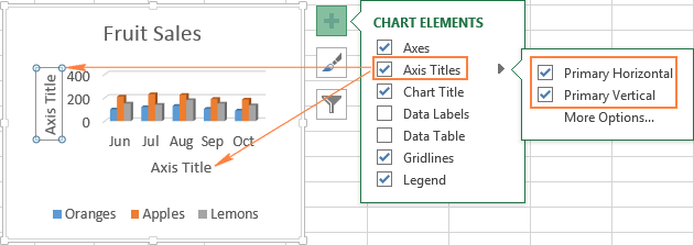
Excel charts: add title, customize chart axis, legend and data labels

How to Create a Run Chart in Excel (2021 Guide) | 2 Free Templates Once there, modify your data markers to make your trend chart so much more visually appealing. In the Format Data Series task pane, switch to the Fill & Line tab. Click "Marker." Select "Marker Options." In the "Type" dropdown menu, customize your marker type. Set the "Size" value to "8."

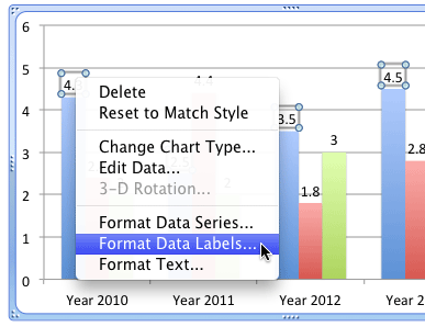
Format Data Label Options in PowerPoint 2011 for Mac

› dynamically-labelDynamically Label Excel Chart Series Lines • My Online ... Sep 26, 2017 · This will open the Format Data Labels pane/dialog box where you can choose ‘Series Name’ and label position; Right, as shown in the image below as shown in the image below for Excel 2013/2016 (Excel 2007/2010 has a slightly different dialog box):

How to Create a Pareto Chart in Excel - Automate Excel

How to mail merge and print labels from Excel - Ablebits In the first step of the wizard, you select Labels and click Next: Starting document near the bottom. (Or you can go to the Mailings tab > Start Mail Merge group and click Start Mail Merge > Labels .) Choose the starting document. Decide how you want to set up your address labels: Use the current document - start from the currently open document.

31 Label Format In Excel - Labels Database 2020

How to Create Labels in Word from an Excel Spreadsheet In this guide, you'll learn how to create a label spreadsheet in Excel that's compatible with Word, configure your labels, and save or print them. Table of Contents 1. Enter the Data for Your Labels in an Excel Spreadsheet 2. Configure Labels in Word 3. Bring the Excel Data Into the Word Document 4. Add Labels from Excel to a Word Document 5.

How to add total labels to stacked column chart in Excel?

Pie Chart in Excel - Inserting, Formatting, Filters, Data Labels Right click on the Data Labels on the chart. Click on Format Data Labels option. Consequently, this will open up the Format Data Labels pane on the right of the excel worksheet. Mark the Category Name, Percentage and Legend Key. Also mark the labels position at Outside End. This is how the chark looks. Formatting the Chart Background, Chart Styles

Share :