38 change data labels in excel chart
excel - How do I update the data label of a chart? - Stack Overflow To build your data labels, somewhere else on your worksheet (conveniently, in the adjacent column would be ideal), use Excel formula to build the desired label string, for example: ="Blue occupies "&TEXT(B3,"0%") Repeat for the other points in the chart. Once you've done that, here's how you link Data Labels to a cell reference (normally, Data ... Create Dynamic Chart Data Labels with Slicers - Excel Campus Feb 10, 2016 · Typically a chart will display data labels based on the underlying source data for the chart. In Excel 2013 a new feature called “Value from Cells” was introduced. This feature allows us to specify the a range that we want to use for the labels. Since our data labels will change between a currency ($) and percentage (%) formats, we need a ...
Custom Data Labels with Colors and Symbols in Excel Charts - [How To ... To apply custom format on data labels inside charts via custom number formatting, the data labels must be based on values. You have several options like series name, value from cells, category name. But it has to be values otherwise colors won't appear. Symbols issue is quite beyond me.
Change data labels in excel chart
How to add or move data labels in Excel chart? - ExtendOffice In Excel 2013 or 2016. 1. Click the chart to show the Chart Elements button . 2. Then click the Chart Elements, and check Data Labels, then you can click the arrow to choose an option about the data labels in the sub menu. See screenshot: In Excel 2010 or 2007. 1. click on the chart to show the Layout tab in the Chart Tools group. See ... How to Add Data Labels in Excel - Excelchat | Excelchat In Excel 2013 and the later versions we need to do the followings; Click anywhere in the chart area to display the Chart Elements button Figure 5. Chart Elements Button Click the Chart Elements button > Select the Data Labels, then click the Arrow to choose the data labels position. Figure 6. How to Add Data Labels in Excel 2013 Figure 7. Format Data Labels in Excel- Instructions - TeachUcomp, Inc. To format data labels in Excel, choose the set of data labels to format. To do this, click the "Format" tab within the "Chart Tools" contextual tab in the Ribbon. Then select the data labels to format from the "Chart Elements" drop-down in the "Current Selection" button group. Then click the "Format Selection" button that ...
Change data labels in excel chart. How to add and customize chart data labels - Get Digital Help Double press with left mouse button on with left mouse button on a data label series to open the settings pane. Go to tab "Label Options" see image to the right. This setting allows you to change the number formatting of the data labels. The image below shows numbers formatted as dates. How to add data labels from different column in an Excel chart? Right click the data series in the chart, and select Add Data Labels > Add Data Labels from the context menu to add data labels. 2. Click any data label to select all data labels, and then click the specified data label to select it only in the chart. 3. How do I replicate an Excel chart but change the data? Oct 18, 2018 · To update the data range, double click on the chart, and choose Change Date Range from the Mekko Graphics ribbon. Select your new data range and click OK in the floating Chart Data dialog box. Your data can be in the same worksheet as the chart, as shown in the example below, or in a different worksheet. Edit titles or data labels in a chart - Microsoft Support The first click selects the data labels for the whole data series, and the second click selects the individual data label. Right-click the data label, and then click Format Data Label or Format Data Labels. Click Label Options if it's not selected, and then select the Reset Label Text check box. Top of Page
How to Change Excel Chart Data Labels to Custom Values? May 05, 2010 · Now, click on any data label. This will select “all” data labels. Now click once again. At this point excel will select only one data label. Go to Formula bar, press = and point to the cell where the data label for that chart data point is defined. Repeat the process for all other data labels, one after another. See the screencast. Step Instructions 1 Start - qfbule.creditorio.eu Step 2: Click the Chart Titles button in Labels group under Layout Tab. Step 3: Select one of two options from the drop down list: Centered Overlay Title: this option will overlay centered title on chart without resizing chart. Here are the steps to create a thermometer chart in Excel: Select the data points. Click the Insert tab. How to change chart axis labels' font color and size in Excel? Sometimes, you may want to change labels' font color by positive/negative/0 in an axis in chart. You can get it done with conditional formatting easily as follows: 1. Right click the axis you will change labels by positive/negative/0, and select the Format Axis from right-clicking menu. 2. Do one of below processes based on your Microsoft Excel ... Add / Move Data Labels in Charts - Excel & Google Sheets Adding Data Labels Click on the graph Select + Sign in the top right of the graph Check Data Labels Change Position of Data Labels Click on the arrow next to Data Labels to change the position of where the labels are in relation to the bar chart Final Graph with Data Labels
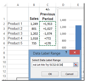
How to Edit Pie Chart in Excel (All Possible Modifications) How to Edit Pie Chart in Excel 1. Change Chart Color 2. Change Background Color 3. Change Font of Pie Chart 4. Change Chart Border 5. Resize Pie Chart 6. Change Chart Title Position 7. Change Data Labels Position 8. Show Percentage on Data Labels 9. Change Pie Chart's Legend Position 10. Edit Pie Chart Using Switch Row/Column Button 11. Change the format of data labels in a chart To get there, after adding your data labels, select the data label to format, and then click Chart Elements > Data Labels > More Options. To go to the appropriate area, click one of the four icons ( Fill & Line , Effects , Size & Properties ( Layout & Properties in Outlook or Word), or Label Options ) shown here. How to Add Data Labels to an Excel 2010 Chart - dummies On the Chart Tools Layout tab, click Data Labels→More Data Label Options. The Format Data Labels dialog box appears. You can use the options on the Label Options, Number, Fill, Border Color, Border Styles, Shadow, Glow and Soft Edges, 3-D Format, and Alignment tabs to customize the appearance and position of the data labels. How to Use Cell Values for Excel Chart Labels - How-To Geek Select the chart, choose the "Chart Elements" option, click the "Data Labels" arrow, and then "More Options." Uncheck the "Value" box and check the "Value From Cells" box. Select cells C2:C6 to use for the data label range and then click the "OK" button. The values from these cells are now used for the chart data labels.
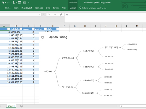
Decision Tree Excel Add-In
How to Customize Your Excel Pivot Chart Data Labels - dummies To add data labels, just select the command that corresponds to the location you want. To remove the labels, select the None command. If you want to specify what Excel should use for the data label, choose the More Data Labels Options command from the Data Labels menu. Excel displays the Format Data Labels pane.

Quickly Create A Variable Width Column Chart In Excel
Excel Chart Data Labels-Modifying Orientation - Microsoft Community You can right click on the data label part then select Format Axis. Click on the Size & Properties tab then adjust the Text Direction or Custom Angle. Thanks, Mike Report abuse 7 people found this reply helpful · Was this reply helpful? Yes No
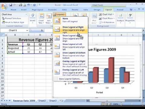
How to add or remove legends, titles or data labels in MS Excel - YouTube
Custom data labels in a chart - Get Digital Help Jan 21, 2020 — Press with right mouse button on on any data series displayed in the chart. · Press with mouse on "Add Data Labels". · Press with mouse on Add ...
How-to Use Data Labels from a Range in an Excel Chart - Excel Dashboard Templates
How to create Custom Data Labels in Excel Charts - Efficiency 365 Right click on any data label and choose the callout shape from Change Data Label Shapes option. Now adjust each data label as required to avoid overlap. Put solid fill color in the labels Finally, click on the chart (to deselect the currently selected label) and then click on a data label again (to select all data labels).

How to Add Data Labels in Excel - Excelchat | Excelchat
Change axis labels in a chart - support.microsoft.com Your chart uses text from its source data for these axis labels. Don't confuse the horizontal axis labels—Qtr 1, Qtr 2, Qtr 3, and Qtr 4, as shown below, with the legend labels below them—East Asia Sales 2009 and East Asia Sales 2010. Change the text of the labels. Click each cell in the worksheet that contains the label text you want to ...

How to Add Data Labels in Excel - Excelchat | Excelchat
Add data labels and callouts to charts in Excel 365 - EasyTweaks.com Step #2: When you select the "Add Labels" option, all the different portions of the chart will automatically take on the corresponding values in the table that you used to generate the chart.The values in your chat labels are dynamic and will automatically change when the source value in the table changes. Step #3: Format the data labels.. Excel also gives you the option of formatting the ...
Post a Comment for "38 change data labels in excel chart"