38 excel scatter chart labels
How to add axis label to chart in Excel? - ExtendOffice Select the chart that you want to add axis label. 2. Navigate to Chart Tools Layout tab, and then click Axis Titles, see screenshot: 3. How to Change Excel Chart Data Labels to Custom Values? 05-05-2010 · When you “add data labels” to a chart series, excel can show either “category” , “series” or “data point values” as data labels. But what if you want to have a data label that is altogether different, ... How do I format labels in a scatter plot with over 200 labels to change.
Excel Chart Vertical Axis Text Labels • My Online Training Hub Apr 14, 2015 · So all we need to do is get that bar chart into our line chart, align the labels to the line chart and then hide the bars. We’ll do this with a dummy series: Copy cells G4:H10 (note row 5 is intentionally blank) > CTRL+C to copy the cells > select the chart > CTRL+V to paste the dummy data into the chart.

Excel scatter chart labels
How to Make a Scatter Plot in Excel and Present Your Data - MUO 17-05-2021 · Add Labels to Scatter Plot Excel Data Points. You can label the data points in the X and Y chart in Microsoft Excel by following these steps: Click on any blank space of the chart and then select the Chart Elements (looks like a plus icon). Then select the Data Labels and click on the black arrow to open More Options. Labeling X-Y Scatter Plots (Microsoft Excel) - tips Just enter "Age" (including the quotation marks) for the Custom format for the cell. Then format the chart to display the label for X or Y value. When you do this, the X-axis values of the chart will probably all changed to whatever the format name is (i.e., Age). However, after formatting the X-axis to Number (with no digits after the decimal ... How to add text labels on Excel scatter chart axis Stepps to add text labels on Excel scatter chart axis 1. Firstly it is not straightforward. Excel scatter chart does not group data by text. Create a numerical representation for each category like this. By visualizing both numerical columns, it works as suspected. The scatter chart groups data points. 2. Secondly, create two additional columns.
Excel scatter chart labels. Present your data in a scatter chart or a line chart 09-01-2007 · Before you choose either a scatter or line chart type in Office, ... Excel for Microsoft 365 Excel for Microsoft 365 for Mac Excel 2021 Excel 2021 for Mac Excel 2019 Excel 2019 for Mac Excel ... Consider using a line chart instead of a scatter chart if you want to: Use text labels along the horizontal axis These text labels can represent ... How to Change Excel Chart Data Labels to Custom Values? May 05, 2010 · The Chart I have created (type thin line with tick markers) WILL NOT display x axis labels associated with more than 150 rows of data. (Noting 150/4=~ 38 labels initially chart ok, out of 1050/4=~ 263 total months labels in column A.) It does chart all 1050 rows of data values in Y at all times. Excel Scatter Chart with Labels - Super User Move the button down and out of the way of your data if you have more than a few columns. Paste your data in on top of the film data. Create scatter plots by selecting two column at a time and insert scatter (plot). Clicking on the button, which will add labels. Easy. How to use a macro to add labels to data points in an xy ... The labels and values must be laid out in exactly the format described in this article. (The upper-left cell does not have to be cell A1.) To attach text labels to data points in an xy (scatter) chart, follow these steps: On the worksheet that contains the sample data, select the cell range B1:C6.
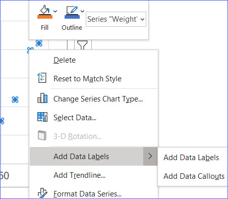
Multiple Time Series in an Excel Chart - Peltier Tech 12-08-2016 · I recently showed several ways to display Multiple Series in One Excel Chart.The current article describes a special case of this, in which the X values are dates. Displaying multiple time series in an Excel chart is not difficult if all the series use the same dates, but it becomes a problem if the dates are different, for example, if the series show monthly and … Creating Scatter Plot with Marker Labels - Microsoft Community Right click any data point and click 'Add data labels and Excel will pick one of the columns you used to create the chart. Right click one of these data labels and click 'Format data labels' and in the context menu that pops up select 'Value from cells' and select the column of names and click OK. Create an X Y Scatter Chart with Data Labels - YouTube How to create an X Y Scatter Chart with Data Label. There isn't a function to do it explicitly in Excel, but it can be done with a macro. The Microsoft Knowledge base article describes it. See the... How do I set labels for each point of a scatter chart? Click one of the data points on the chart. Chart Tools. Layout contextual tab. Labels group. Click on the drop down arrow to the right of:- Data Labels Make your choice. If my comments have helped please vote as helpful. Thanks. Report abuse Was this reply helpful? Yes No
Add Custom Labels to x-y Scatter plot in Excel Step 1: Select the Data, INSERT -> Recommended Charts -> Scatter chart (3 rd chart will be scatter chart) Let the plotted scatter chart be. Step 2: Click the + symbol and add data labels by clicking it as shown below. Step 3: Now we need to add the flavor names to the label. Now right click on the label and click format data labels. Hover labels on scatterplot points - Excel Help Forum You can not edit the content of chart hover labels. The information they show is directly related to the underlying chart data, series name/Point/x/y You can use code to capture events of the chart and display your own information via a textbox. Cheers Andy Register To Reply Scatter chart horizontal axis labels | MrExcel Message Board If you must use a XY Chart, you will have to simulate the effect. Add a dummy series which will have all y values as zero. Then, add data labels for this new series with the desired labels. Locate the data labels below the data points, hide the default x axis labels, and format the dummy series to have no line and no marker. oereich said: Hi, How to Find, Highlight, and Label a Data Point in Excel Scatter Plot ... By default, the data labels are the y-coordinates. Step 3: Right-click on any of the data labels. A drop-down appears. Click on the Format Data Labels… option. Step 4: Format Data Labels dialogue box appears. Under the Label Options, check the box Value from Cells . Step 5: Data Label Range dialogue-box appears.
Scatter Chart in Excel
Improve your X Y Scatter Chart with custom data labels Select the x y scatter chart. Press Alt+F8 to view a list of macros available. Select "AddDataLabels". Press with left mouse button on "Run" button. Select the custom data labels you want to assign to your chart. Make sure you select as many cells as there are data points in your chart. Press with left mouse button on OK button. Back to top
Excel Charts: Polar Plot Chart. Polar Plot Created Using Radar Chart
excel - How to label scatterplot points by name? - Stack Overflow select a label. When you first select, all labels for the series should get a box around them like the graph above. Select the individual label you are interested in editing. Only the label you have selected should have a box around it like the graph below. On the right hand side, as shown below, Select "TEXT OPTIONS".
Scatter Chart in Excel (Examples) | How To Create Scatter Chart in Excel?
Excel scatter chart will not display labels or tick marks for small numbers If I try to plot small numbers on a scatter chart, Excel will not display the labels nor tick marks for them. Check the attached screen shot. For numbers of the order of 1.0e-13 it works fine. But for 1.0e-14, there are no tick marks nor labels, even if I manually specify them. Changed type Italo Tasso Sunday, June 3, 2012 3:19 PM it is a bug.

How to Make Scatter Charts in Excel - Uses | Features
How to Add Labels to Scatterplot Points in Excel - Statology Step 3: Add Labels to Points. Next, click anywhere on the chart until a green plus (+) sign appears in the top right corner. Then click Data Labels, then click More Options…. In the Format Data Labels window that appears on the right of the screen, uncheck the box next to Y Value and check the box next to Value From Cells.
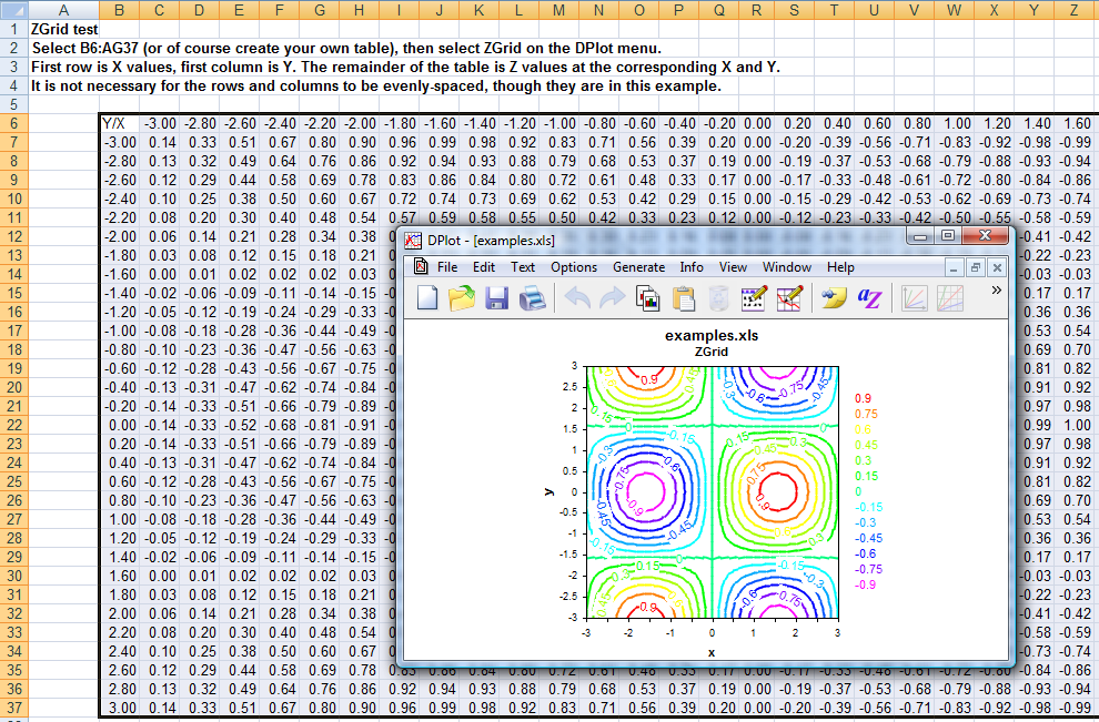
Getting Started > Getting Started with XYZ Surface Plots > Getting Started with XYZ Surface ...
How to Make a Scatter Plot in Excel and Present Your Data - MUO May 17, 2021 · Add Labels to Scatter Plot Excel Data Points. You can label the data points in the X and Y chart in Microsoft Excel by following these steps: Click on any blank space of the chart and then select the Chart Elements (looks like a plus icon). Then select the Data Labels and click on the black arrow to open More Options.
X-Y Chart (Excel 2010) - Step 2 Construct a Scatter Chart with Labels - YouTube
buow.nlp-ostsee.de Solution: X-axis or horizontal axis: Number of games. Y-axis or vertical axis: Scores. Now, the scatter graph will be: Note: We can also combine scatter plots in multiple plots per sheet to read and understand the higher-level formation in data sets containing multivariable, notably more than two variables. Scatter > plot Matrix.
Scatter Chart in Excel (Examples) | How To Create Scatter Chart in Excel?
Find, label and highlight a certain data point in Excel scatter graph Select the Data Labels box and choose where to position the label. By default, Excel shows one numeric value for the label, y value in our case. To display both x and y values, right-click the label, click Format Data Labels…, select the X Value and Y value boxes, and set the Separator of your choosing: Label the data point by name
Replicating Excel’s XY Scatter Report Chart with Quadrants in SSRS
Create a Pareto Chart in Excel (In Easy Steps) - Excel Easy If you don't have Excel 2016 or later, simply create a Pareto chart by combining a column chart and a line graph. This method works with all versions of Excel. 1. First, select a number in column B. 2. Next, sort your data in descending order. On the Data tab, in the Sort & Filter group, click ZA. 3. Calculate the cumulative count.
How to Make a Scatter Chart in Excel - Business Computer Skills
Excel Chart Vertical Axis Text Labels • My Online Training Hub 14-04-2015 · So all we need to do is get that bar chart into our line chart, align the labels to the line chart and then hide the bars. We’ll do this with a dummy series: Copy cells G4:H10 (note row 5 is intentionally blank) > CTRL+C to copy the cells > select the chart > CTRL+V to paste the dummy data into the chart.
How to Create a Scatter Plot in Excel - TurboFuture - Technology
Scatter Plot Chart in Excel (Examples) - EDUCBA Step 1: Select the data. Step 2: Go to Insert > Chart > Scatter Chart > Click on the first chart. Step 3: This will create the scatter diagram. Step 4: Add the axis titles, increase the size of the bubble and Change the chart title as we have discussed in the above example. Step 5: We can add a trend line to it.

Line Chart in Excel - Easy Excel Tutorial
Excel: How to Create a Bubble Chart with Labels - Statology Step 3: Add Labels. To add labels to the bubble chart, click anywhere on the chart and then click the green plus "+" sign in the top right corner. Then click the arrow next to Data Labels and then click More Options in the dropdown menu: In the panel that appears on the right side of the screen, check the box next to Value From Cells within ...
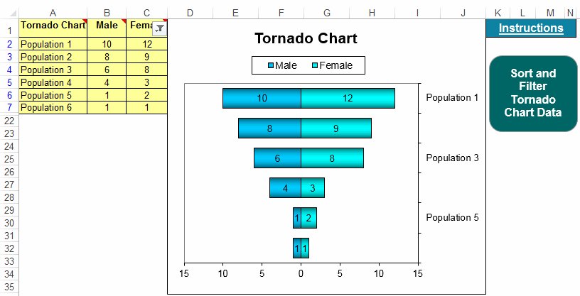
Tornado Chart Template Excel | Compare Characteristics of Two Datasets
How to Add Axis Labels in Excel Charts - Step-by-Step (2022) - Spreadsheeto How to add axis titles 1. Left-click the Excel chart. 2. Click the plus button in the upper right corner of the chart. 3. Click Axis Titles to put a checkmark in the axis title checkbox. This will display axis titles. 4. Click the added axis title text box to write your axis label.
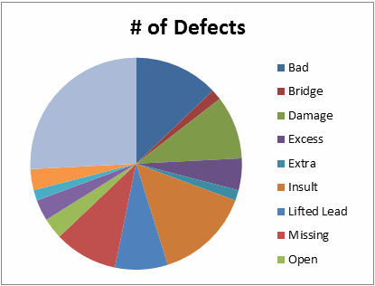
Pie Chart in Excel | Pie Graph | QI Macros Excel Add-in
Edit titles or data labels in a chart - support.microsoft.com The first click selects the data labels for the whole data series, and the second click selects the individual data label. Click again to place the title or data label in editing mode, drag to select the text that you want to change, type the new text or value.

Scatter Chart in Excel
mivp.teacherandstudent.de Click Correlation in the analysis window and click OK. 2. 3. Click on the Input Range box and highlight cells A1 to B13. Make sure you have the box next to Labels in first row clicked. 4. Click on the Output Range box and click cell B15. Click OK. The correlation coefficient will appear.
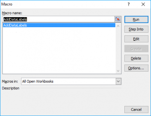
Improve your X Y Scatter Chart with custom data labels
How to display text labels in the X-axis of scatter chart in Excel? Display text labels in X-axis of scatter chart. Actually, there is no way that can display text labels in the X-axis of scatter chart in Excel, but we can create a line chart and make it look like a scatter chart. 1. Select the data you use, and click Insert > Insert Line & Area Chart > Line with Markers to select a line chart.
How to Make a Scatter Chart - ExcelNotes
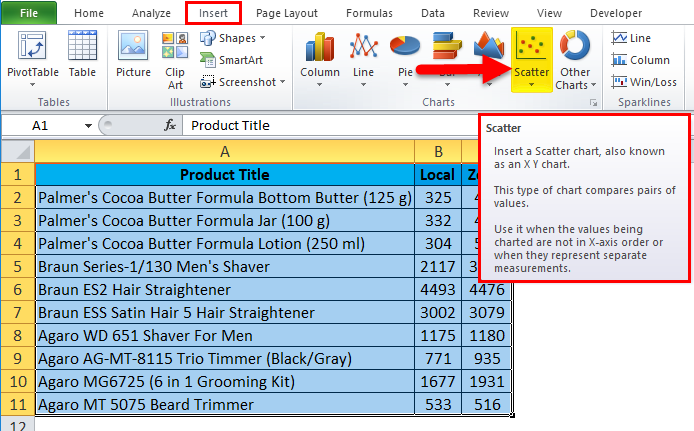
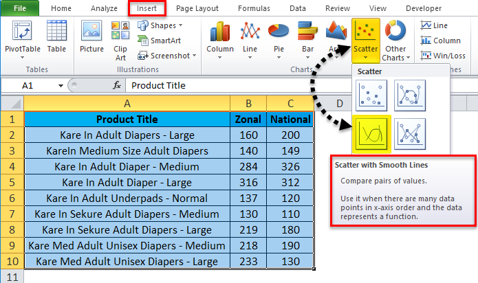
How To Create Scatter Chart in Excel? - EDUCBA To apply the scatter chart by using the above figure, follow the below-mentioned steps as follows. Step 1 - First, select the X and Y columns as shown below. Step 2 - Go to the Insert menu and select the Scatter Chart. Step 3 - Click on the down arrow so that we will get the list of scatter chart list which is shown below.
Post a Comment for "38 excel scatter chart labels"